Large-scale-structure sonifications

Click on each square for a sonification of that field.
The waveforms that produce each sound are what a phonograph needle would encounter going through that representation of the density field at a speed of 3 Gpc/sec. 3 Gpc is about the distance to the farthest galaxies ever seen (by us) in the universe. This speed can also be expressed as 9 billion light-years per second, or 300 quadrillion (3x10^17) times the speed of light.

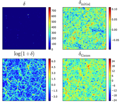
The density used is the average density measured in 2 Mpc/h (about 9 million light-years) cubic cells, in the Millennium simulation, a very high-resolution N-body simulation of large-scale structure formation in the universe.

delta (δ) is the overdensity, density/(mean density) - 1.
log(1+delta) is the natural logarithm of (density/(mean density)).
delta_Gauss is the "Gaussianized" delta, in which the rank of cell densities in the grid is preserved, but a Gaussian (normal) distribution of delta is imposed.
delta_initial is delta in the initial conditions of the simulation when the universe was 1/128 of its current size, not long after the cosmic microwave background was emitted.

The starkest difference among the sounds is, just as in the visualization, between delta and the other three fields. The similarity of the three other fields' sounds suggests a similarity in their spatial power spectra. This points to the scientific value of the log(1+δ) and Gaussianization transforms (not just for sonifications and visualizations), which we explore in the paper Rejuvenating the Matter Power Spectrum: Restoring Information with a Logarithmic Density Mapping.

The sound waveforms are produced by going on a very squiggly path through the 3D grid, ordered along a Peano-Hilbert space-filling curve, used in the Millennium simulation data structures. This type of path is arguably good for sonification, since it ensures that the sound encountered in a small span of time comes from a small spatial region in the grid. Going on a straight-line path would make the sound be composed of very faraway regions even in a small timespan, which reduces the physical meaning of the sound. Note that this curve has excursions in all three dimensions, and comes from a different region of the simulation than the one visualized above. The path taken is 256^2 cells long, representing 1/256 of the total datacube.

To turn the waveforms into sounds, we used the python wave.py package. We play each waveform at full volume, i.e. setting the maximum and minimum amplitudes to the maximum and minimum values in the data. The frame rate is quite low, only 1kHz; thus, this is the maximum possible frequency in the sound.

Image, sounds, and text (c) Mark Neyrinck, Istvan Szapudi, and Alex Szalay. Thanks to Ben Granett for the phonograph analogy. The Millennium Simulation databases used for this project and the web application providing online access to them were constructed as part of the activities of the German Astrophysical Virtual Observatory.